Neural Networks from Scratch — part 3 Multiple inputs and Activations

Welcome for a third time! This guide will improve our neural network from the previous part by allowing for each neuron to have multiple inputs as we as activation functions.

Where we left off

Here was our final code:

Cost Function

class MSE:
    def forward(self, a, y):
        return np.power(a - y, 2).mean()

    def backward(self, a, y):
        return 2 * (a - y)

Neuron

class Neuron:
    def __init__(self):
        # Initializing random weight and bias
        self.w = np.random.randn(1) * 0.01
        self.b = np.random.randn(1) * 0.01

    def forward(self, x):
        # Storing the x value for later use
        self.input = x

        # Equation of straight line
        self.z = self.input * self.w + self.b
        return self.z

    def backward(self, error, learning_rate):
        # Getting the derivatives
        dzdw = self.input
        dzdb = 1

        # These are the first and second terms of the gradient vector
        dLdw = -error * dzdw
        dLdb = -error * dzdb

        # Updating our weight and bias
        self.w += learning_rate * dLdw
        self.b += learning_rate * dLdb

        # The error of the previous layer
        return self.w

Network

class Network:
    def __init__(self, neurons, loss_function):
        self.neurons = neurons
        self.loss_function = loss_function

    def forward(self, x):
        for n in self.neurons:
            x = n.forward(x)
        return x

    def backward(self, error, learning_rate):
        for i in range(len(self.neurons), 0, -1):
            error = self.neurons[i - 1].backward(error, learning_rate)

    def train(self, training_data, training_labels, learning_rate, epochs):
        for epoch in range(epochs):
            total_error = 0

            # Running the training
            for i in range(len(training_data)):
                a = self.forward(training_data[i])
                total_error += self.loss_function.forward(a, training_labels[i])
                self.backward(
                    self.loss_function.backward(a, training_labels[i]), learning_rate
                )

            if epoch % (epochs / 10) == 0:
                print(
                    f"epoch = {epoch}, error = {round(total_error / len(training_data), 3)}"
                )

Adding activations

Last time, we saw that since all neurons are just linear functions, not matter how many we chain together, the output will still be a linear function. We need to add some nonlinearity to allow for more complex patterns and models to be learnt.

Nonlinearity in neural networks is created through the activation functions.

Suppose we have a single neuron. Its output looks like this:

We add another equation to the neuron:

Where f is any non-linear function you want: Quadratic, sigmoid, exponential, etc. In this way, the final output of our neuron is no longer just a straight line.

Let’s try modelling that quadratic equation with the help of activations.

Our curve looked like this:

x = np.array([i for i in range(1, 11)])
y = x**2 + 6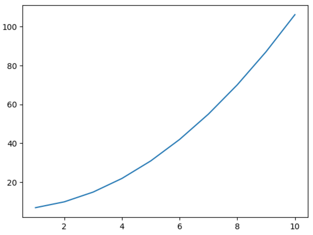

Adding the Quadratic activation class

Just like how we made a class for the MSE error with both forward and backward functions, we need to make the same for the Quadratic activation.

class Quadratic:
    def forward(self, x): return x**2
    
    def backward(self, x): return 2*x

The derivative of the Quadratic is just 2x, so the math is pretty simple here.

Gradient descent with activation functions

Gradient descent with activation functions is mostly the same, just with one extra equation.

Note: If you’ve forgotten the gradient descent calculation we did in the previous guides, please go through them again. Otherwise this will seem very complicated

Suppose our network had 2 neurons chained together. The equations for the forward pass of our network will look like this:

Notice how we no longer use z1 for the calculation of z2 but rather a1. Now we look at the gradient descent. First remember that our loss is calculated through MSE, so its gradient will be twice the difference between the predicted y and the actual y:

Then we propagate it to every variable using the chain rule:

Remember that z2 and a2 are the same (this means the activation function of the second neuron is just the identity function f(x) = x. So the partial of a2 w.r.t (with respect to) z2 will be 1.

But now, to calculate the gradient for the first neuron, we have to remember that the output of the neuron was passed through an activation function to get a1, so we have an extra variable to account for:

Now, since have the gradient for a1, we can calculate the gradient of z1. This will be the derivative of the activation function:

Since the equation was getting too big, I did not simplify it. Basically, to get the influence of z1 on L, we need to first get the influence of z1 on a1 and then the influence of a1 on L. We calculated the latter part in the previous equation and the influence of z1 on a1 is the derivative of the quadratic.

Notice one thing: To calculate the partial of a1 w.r.t z1, we need to not only calculate the derivative of the quadratic function but also input it with the value of z1. This means we need to store our value of z when calculating the forward pass.

Finally, we have the weight and the bias. This is the same as for the second neuron:

Updating the code

Now that the hard part is over, we can simply update our Network class. First, we’ll update the __init__ function of the network class to store the activation function. But we’re storing an entire list of activation functions. This is because we can have multiple neurons, each with its own activation.

class Network:
    def __init__(self, neurons, activations, loss_function):
        self.neurons = neurons
        self.z = []
        self.activations = activations
        self.loss_function = loss_function

Notice that we’re also storing the output of each neuron z in a list self.z.

Then, in our forward pass, we’ll run the input through n.forward(), but after that, we also need to run it through the right activation function. Here is a little trick in Python. It’s called enumerate. Enumerate combines the loops for n in self.neurons and for i in range(len(self.neurons)). So, we have both the index of each neuron and the neuron itself too. We need to neuron to run the forward function, but we also need the index of the neuron to get the right activation from our list of activations.

def forward(self, a):
    for i, n in enumerate(self.neurons):
        # Forward pass of the neuron
        z = n.forward(a)
        self.z.append(z)

        # Getting the activation function and running its forward
        a = self.activations[i].forward(z)

    return a

Our backward pass also looks the same, except for one line:

def backward(self, error, learning_rate):
        for i in range(len(self.neurons), 0, -1):
            # Passing the error through the activation
            error *=  self.activations[i - 1].backward(self.z[i - 1])

            # Passing the error through each neuron
            error = self.neurons[i - 1].backward(error, learning_rate)

Before sending the error off to the neuron, we first multiply it with the backward pass of the activation function. Remember this equation:

The partial of L w.r.t to a1 is the error we get for each neuron. Then we have to multiply it with the derivative of the quadratic function. We do this with the line:

error *=  self.activations[i - 1].backward(self.z[i - 1])

Notice we’re also indexing the self.z list. So this means that if we have 3 neurons, each with a quadratic activation, we can properly run the backwards pass for each of them.

The entire code looks like this:

class Network:
    def __init__(self, neurons, activations, loss_function):
        self.neurons = neurons
        self.z = []
        self.activations = activations
        self.loss_function = loss_function

    def forward(self, a):
        for i, n in enumerate(self.neurons):
            z = n.forward(a)
            self.z.append(z)
            a = self.activations[i].forward(z)

        return a

    def backward(self, error, learning_rate):
        for i in range(len(self.neurons), 0, -1):
            error *=  self.activations[i - 1].backward(self.z[i - 1])
            error = self.neurons[i - 1].backward(error, learning_rate)

    def train(self, training_data, training_labels, learning_rate, epochs):
        for epoch in range(epochs):
            total_error = 0

            # Running the training
            for i in range(len(training_data)):
                a = self.forward(training_data[i])
                total_error += self.loss_function.forward(a, training_labels[i])
                self.backward(self.loss_function.backward(a, training_labels[i]), learning_rate)

            if epoch % (epochs/10) == 0:
                print(f"epoch = {epoch}, error = {round(total_error / len(training_data), 3)}")

The code for each neuron remains the same. This is because the error that is sent to each neuron is the derivative of L w.r.t z. The only thing we did was add something after that calculation, so we don’t need to update anything before it.

Testing the network

network = Network([Neuron()], [Quadratic()], MSE())
network.train(x, y, learning_rate=0.001, epochs = 10000)
pred = [network.forward(i) for i in x]
plt.plot(x, y)
plt.plot(x, pred)
plt.show()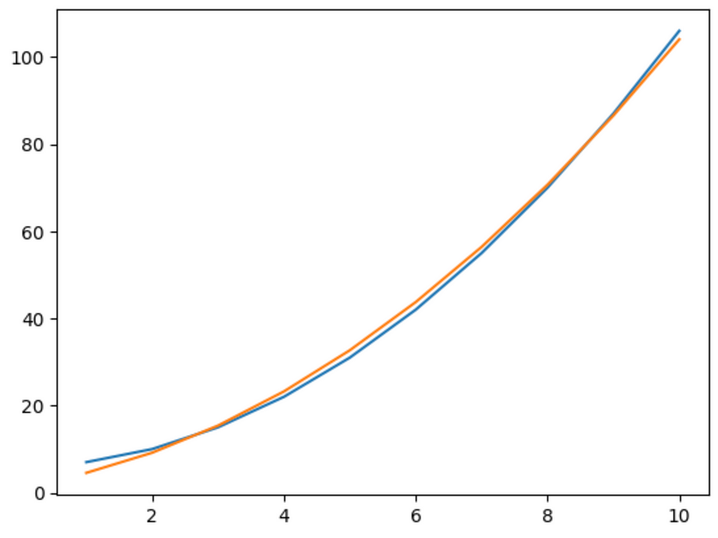

And there we go. It does a pretty good job of modelling a quadratic relation. Since this is a simple model, we can increase the learning rate to 0.01 and it will most likely perfectly match the graph.

Why need multiple inputs

Let’s take a step back and reflect on what we did. At first, we needed to model a linear relationship, we did that through a straight-line equation in the neuron. Then we needed to model a quadratic relation, so we added a quadratic activation function. Does that mean for each new type of relation, we need a new custom activation function? That seems like too much work. What if there was a way to have a single network that could learn any relation we put in?

We do this using a technique known as the sliding window. Basically, instead of taking x as the input and producing a y as the output. We only look at y. We take in the previous n values of y and try to predict the next one. This could mean using the previous 5 values to predict the next value or using the previous 10 values to predict the next 5. n here is called the window size.

Let’s try to convert our data into this format.

We begin with two arrays:

import numpy as np
x_set = np.array([i for i in range(1, 101)]) # x values from 1 to 100
y_set = np.sin(x_set) + 6

These are the same as last time, we create a range of values for x and use an equation to generate all the values of y, in this case, the equation for sin(x)+6. But I called them x_set and y_set, because they are the set of values we’re using to generate our actual input and output.

To generate our x and y, we first initialise our window_size. This represents how many previous values of y are we going to use to predict the next one.

I’d like to remind you how list indexing works in Python. If I say list[1:3] . It’s going to take the elements at position 1 and position 2. Python list indexing includes the first number but excludes the next number.

Suppose our y looks like this:

y = [0, 1, 2, 3, 4, 5, 6, 7, 8, 9, 10, 11, 12, 13, 14, 15]

Suppose we start at position 4. How do we take the next 5 values?

We can do that using y[4:4+5]. This will take the 4th, 5th, 6th, 7th, and 8th elements. It will exclude the (4+5 = 9)th element. Then, to take the next element, I simply query y[4+5].

What we just did was the sliding window technique. Starting at position 4, we took 5 values of y as our input and then the next value of y as our output. If we do this for every index, we get a whole bunch of windows:

window_size = 5
x = []
y = []

for i in range(0, len(y_set) - window_size):
    x.append(y_set[i:i+window_size])
    y.append(y_set[i+window_size])

x = np.array(x)
y = np.array(y)

To understand why we used that particular range, think of this logic. We can’t query something outside the bounds of the array. Remember that the range function also excludes the final value. So, if we use range(0, len(y_set) — window_size. Our final value of i will be len(y_set) — window_size — 1. That means the final value of our y query will be:

y_set[i+window_size]

Substituting the value of i :

y_set[len(y_set) - window_size - 1]

which is

y_set[len(y_set) - 1]

This is precisely the last element of the array.

As a sanity check, see what x[0] and y[0] are. They should be the first 5 elements of our y values and 6th element:

x[0] = array([ 1.62782875,  0.55344516,  0.77406597, -1.87440279, -1.17660632]
y[0] = -0.10180537571676801

Our job now is to update our neurons so that they take in the 5 values in x and output the predictions for y.

Updating the neuron

Each neuron is now taking multiple inputs. So we need that many weights. We update the __init__ function like this:

class Neuron:
    def __init__(self, input_size):
        # Initializing random weight and bias
        self.w = np.random.randn(input_size) * 0.01
        self.b = np.random.randn(1) * 0.0

Think of the weights and the inputs as vectors. In our case, the weight is a vector with 5 elements:

and the input is a vector of 5 elements:

We need to multiply each input element with the respective weight:

The dot product in linear algebra precisely does this. Finally, we also need to add the bias:

    def forward(self, x):
        # Storing the x value for later use
        self.input = x

        self.z = np.dot(self.input, self.w) + self.b
        return self.z

Now for the backward part. Remember in the previous guide we found how to compute the gradient of the weight for each neuron as:

That was because the equation was:

Now the equation is:

So, each weight’s gradient will simply be:

If we find this gradient for each weight and combine them in the form of a vector, we get:

We can neatly write this equation as:

Where W and X are vectors. Notice this is the same as our previous equation for a single weight:

Since Numpy already handles these changes well, we don’t need to do anything new. So our backwards function remains the same.

    def backward(self, error, learning_rate):
        # Getting the derivatives
        dzdw = self.input
        dzdb = 1
        dzdprev = self.w

        # These are the first and second terms of the gradient vector
        dLdw = -error * dzdw
        dLdb = -error * dzdb


        # Gradient clipping
        dLdw = np.clip(dLdw, -1, 1)
        dLdb = np.clip(dLdb, -1, 1)

        # Updating our weight and bias
        self.w += learning_rate * dLdw
        self.b += learning_rate * dLdb

        return dzdprev

Final code

class Neuron:
    def __init__(self, input_size):
        # Initializing random weight and bias
        self.w = np.random.randn(input_size) * 0.01
        self.b = np.random.randn(1) * 0.01

    def forward(self, x):
        # Storing the x value for later use
        self.input = x

        self.z = np.dot(self.input, self.w) + self.b
        return self.z

    def backward(self, error, learning_rate):
        # Getting the derivatives
        dzdw = self.input
        dzdb = 1
        dzdprev = self.w

        # These are the first and second terms of the gradient vector
        dLdw = -error * dzdw
        dLdb = -error * dzdb


        # Gradient clipping
        dLdw = np.clip(dLdw, -1, 1)
        dLdb = np.clip(dLdb, -1, 1)

        # Updating our weight and bias
        self.w += learning_rate * dLdw
        self.b += learning_rate * dLdb

        return dzdprev

class Network:
    def __init__(self, neurons, activations, loss_function):
        self.neurons = neurons
        self.z = []
        self.activations = activations
        self.loss_function = loss_function

    def forward(self, a):
        for i, n in enumerate(self.neurons):
            z = n.forward(a)
            self.z.append(z)
            a = self.activations[i].forward(z)

        return a

    def backward(self, error, learning_rate):
        for i in range(len(self.neurons), 0, -1):
            error = error * self.activations[i - 1].backward(self.z[i - 1])
            error = self.neurons[i - 1].backward(error, learning_rate)

    def train(self, training_data, training_labels, learning_rate, epochs):
        for epoch in range(epochs):
            total_error = 0

            # Running the training
            for i in range(len(training_data)):
                a = self.forward(training_data[i])
                total_error += self.loss_function.forward(a, training_labels[i])
                self.backward(self.loss_function.backward(a, training_labels[i]), learning_rate)

            if epoch % (epochs/10) == 0:
                print(f"epoch = {epoch}, error = {round(total_error / len(x), 3)}")

Testing it out:

network = Network([Neuron(x.shape[1])], [Identity()], MSE())
network.train(x, y, learning_rate=0.01, epochs = 1000)
pred = [network.forward(i)[0] for i in x]
plt.plot(x_set[x.shape[1]:], y_set[x.shape[1]:], label='actual')
plt.plot(x_set[x.shape[1]:], pred, label='predicted')
plt.legend()
plt.show()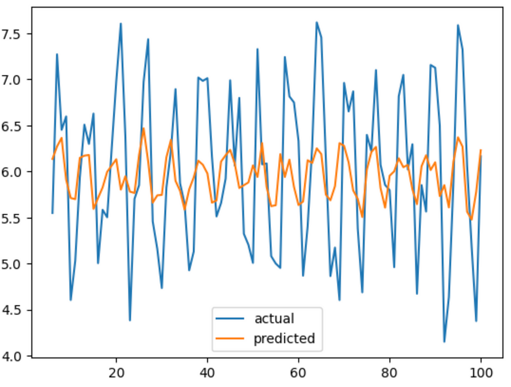

Well, it got the right shape. It’s going up in the right places and going down in the right places. But it doesn’t have the same amplitude. We can kinda cheat it by normalizing our data. This means just reducing the scale of it and centring it around 0.

x_set = np.array([i for i in range(1, 101)])
y_set = np.sin(x_set) + 6 + np.random.randn(x_set.shape[0]) * 0.5


# Normalization
x_set = (x_set - np.mean(x_set)) / np.std(x_set)
y_set = (y_set - np.mean(y_set)) / np.std(y_set)

step_size = 5
x = []
y = []
for i in range(0, len(x_set) - step_size):
    x.append(y_set[i:i+step_size])
    y.append(y_set[i+step_size])

x = np.array(x)
y = np.array(y)

Now if we run the training:

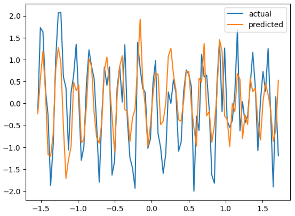
This is a lot closer. Look at that! we didn’t even put any activation function in and it still got the right graph. Although its not that accurate. If we try to add one more neuron, we’d need to decrease the learning rate to 0.001 since this is a more complex model. We’ll also need to increase the number of epochs.

network = Network([Neuron(x.shape[1]), Neuron(1)], [ReLU(), Identity()], MSE())
network.train(x, y, learning_rate=0.001, epochs = 10000)
pred = [network.forward(i)[0] for i in x]
plt.plot(x_set[x.shape[1]:], y_set[x.shape[1]:], label='actual')
plt.plot(x_set[x.shape[1]:], pred, label='predicted')
plt.legend()
plt.show()

It seems… worse? Well, it still got the right direction, sort of, but again, the amplitude is so little. It also took a lot longer to train. This is because our gradient descent algorithm is the most primitive you could’ve had. Modern neural networks have a more complex gradient descent algorithm called “ADAM (Adaptive Moment Estimation)”.

Conclusion

In this guide, we’ve expanded our neural network to handle multiple inputs and incorporate activation functions, allowing for more complex relationships to be modelled. Until now, we only have a single neuron in each layer. In the next guide, we’ll look into creating the layer class. Keep experimenting with different architectures and activation functions to see how they affect your model’s performance! Happy coding!